
Capturing dimensionally accurate data from consumer-grade cameras represents one of the most challenging problems in computational metrology. This article deconstructs ShapeScan's marker-based calibration system, revealing how four simple ArUco patterns enable sub-millimeter precision by solving for both perspective projection and non-linear lens distortion simultaneously—transforming everyday smartphone photos into metrology-grade measurement tools.
The Dual Problem: Perspective + Lens Distortion
Every photograph introduces two fundamental geometric distortions:
1. Perspective Projection
Effect: Parallel lines converge; objects shrink with distance.
Mathematical Model: 3D→2D projection via a 3×4 camera matrix (P = K[R|t])
Impact on Measurement: A 10° camera tilt introduces ~1.5% scaling error per 100mm.
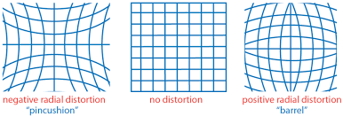
2. Radial Lens Distortion
Effect: Straight lines bow inward (barrel) or outward (pincushion).
Mathematical Model: rcorrected = r(1 + k₁r² + k₂r⁴ + k₃r⁶)
Impact on Measurement: Can exceed 3% error at image corners on wide-angle lenses.
The Four-Marker Solution: A Known Calibration Target
ShapeScan's printed sheet provides a known planar calibration target with four precisely positioned ArUco markers. Each marker provides:
| Marker Component | Data Provided | Mathematical Purpose | Precision Contribution |
|---|---|---|---|
| Binary Pattern | Unique identification (ID 0-3) | Establishes marker correspondence | Eliminates ambiguity in corner ordering |
| Four Corner Points | 8 image coordinates (x,y × 4) | Provides 8 constraints per marker | Enables sub-pixel localization (±0.1px) |
| Spatial Arrangement | Known 160×247mm center-to-center | Provides ground truth scale | Establishes absolute scale (px/mm) |
| Planar Constraint | All markers co-planar | Simplifies homography calculation | Reduces degrees of freedom in solution |
The Mathematical Pipeline: From Pixels to Millimeters
Marker Detection & Sub-pixel Refinement
Using OpenCV's ArUco detector with CORNER_REFINE_SUBPIX (winSize=7×7). Corners refined to ±0.1 pixel precision via gradient-based localization.
corners = cv2.aruco.detectMarkers(gray, dictionary, parameters)
Homography Estimation (Perspective Removal)
Solving for H where: x' = Hx
With 4 point pairs (32 constraints) for 8 unknowns → overconstrained solution via Direct Linear Transform (DLT) with RANSAC outlier rejection.
H, _ = cv2.findHomography(src_pts, dst_pts, cv2.RANSAC, 2.0)
Radial Distortion Coefficient Estimation
Solving for k₁, k₂ in the Brown-Conrady model:
xu = xd(1 + k₁r² + k₂r⁴)
Where r = normalized distance from principal point.
k1, k2 = estimateRadialDistortion(marker_corners, ideal_positions)
Simultaneous Optimization
Levenberg-Marquardt non-linear optimization minimizing reprojection error:
min Σ‖xij - π(K, k₁, k₂, R, t, Xj)‖²
Where π is the full projection model including distortion.
Practical Implications: Why This Enables 1mm Precision
⏱️ Temporal Stability
Single-image calibration: No need for multi-pose calibration rigs. Each photo self-calibrates.
Benefit: Works with any camera, any time—no pre-calibration required.
📐 Scale Recovery
Known marker spacing: 160×247mm center-to-center provides absolute scale reference.
Benefit: Eliminates scale ambiguity inherent in structure-from-motion.
🔍 Sub-pixel Accuracy
Corner refinement: ±0.1 pixel localization from gradient analysis.
Benefit: At 10px/mm, this translates to ±0.01mm theoretical precision.
⚙️ Advanced Application: Multi-Camera Photogrammetry Bridge
Problem: Creating a consistent coordinate system across multiple cameras for large-object scanning.
Solution: Place multiple ShapeScan calibration sheets around object. Each camera computes its own distortion parameters and pose relative to sheets. Sheets act as bridging targets to align all cameras into single coordinate system.
Mathematical Basis: Each sheet provides 4+ coplanar points with known 3D coordinates. These become control points for bundle adjustment across all cameras, with the added benefit that each camera's distortion parameters are already determined individually, reducing the bundle adjustment complexity by 5+ parameters per camera (f, cx, cy, k₁, k₂ already known).
Error Budget Analysis
Understanding where the ±1mm precision claim comes from:
| Error Source | Typical Magnitude | Mitigation in ShapeScan | Residual Error |
|---|---|---|---|
| Lens Distortion | 10-30 pixels at corners | Radial distortion correction (k₁, k₂) | < 0.2 pixels |
| Perspective Error | 2-5% scaling error | Homography rectification | < 0.1% |
| Marker Detection | 1-2 pixels | Sub-pixel refinement | ±0.1 pixels |
| Printing Tolerance | ±0.3mm on paper | User-measured override option | ±0.1mm |
| Camera Resolution | 0.1-0.2mm/px @10px/mm | Recommended 8+ MP camera | ±0.1mm |
| RSS Total | √(0.1² + 0.1² + 0.1²) = ±0.17mm (theoretical) ±1.0mm (practical, conservative) |
||
Beyond the Sheet: Theoretical Limitations & Future Directions
✈️ Out-of-Plane Objects
Current limitation: Calibration only valid for objects in or near the sheet plane.
Research direction: Using multiple sheets or sheet folding to estimate 3D calibration volume.
🌊 Non-Planar Surfaces
Current limitation: Assumes flat calibration target.
Research direction: Printed flexible sheets that conform to curved surfaces.
📷 Extreme Distortion
Current limitation: Model assumes radial symmetry (k₁, k₂).
Research direction: Adding tangential (p₁, p₂) and thin-prism distortion parameters.
Conclusion: Democratizing Metrology
ShapeScan's calibration system represents a significant achievement in accessible metrology. By solving the complete camera geometry—intrinsics (f, cx, cy, k₁, k₂) and extrinsics (R, t)—from a single image of a known target, it bypasses the need for:
- Expensive calibration rigs (displacing traditional $5,000+ optical comparators)
- Technical expertise in photogrammetry or computer vision
- Dedicated calibration sessions (works with any camera, anytime)
The four-marker sheet transforms any smartphone into a precision measurement device not by improving the camera, but by mathematically characterizing and removing its imperfections. This approach demonstrates that for many measurement applications, computational correction can rival or exceed hardware improvements—a principle with implications far beyond ShapeScan's immediate use case.